Impacts of commodity prices and governance on the expansion of tropical agricultural frontiers

Data processing

We conducted a subnational analysis using a mesoregion as the unit of observation. We refer to these mesoregions as agro-ecological zone (AEZ)-country units. These regions are obtained by intersecting spatial information on the Global AEZs (GAEZ; https://gaez.fao.org/)⁵³ and national administrative boundaries for the whole world from the Database of Global Administrative Areas (https://gadm.org/index.html). Agro-ecological zones are regions with similar natural features like climate, soil, and terrain, influencing crop-specific agricultural potential. We identified 876 AEZ-country regions (see Fig. S1 for a graphic representation) based on the overview of GAEZ by Plevin et al.⁵⁴, from which we selected tropical areas. We chose these AEZ-country observations as they have been subject to deforestation in the current century (visit https://globalforestwatch.org/ for a spatially explicit assessment on deforestation). Finally, 267 mesoregions were identified, as depicted in Fig. 6. The fundamental reason for using this level of analysis is that mesoregions are the units used in several applications of global CGE models such as those in the GTAP family^22,55,56. Thus, the calculation of individual elasticities for these units of observation offers information to calibrate land use change in these CGE models (Fig. 6).

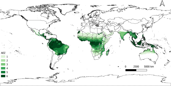
Tropical AEZ-country regions. Each mesoregion refers to the intersection between agro-ecological zones and national administrative boundaries. Shades of green reflect the different tropical zones considered for data analysis. We do not include those with a desert climate in the final econometric estimation, i.e., AEZ 1.

We measured agricultural land, which is the outcome variable in the empirical analysis, as the share of the total land in an AEZ-country observation. It is common to use only cropland as a response variable to analyze drivers of land supply and calculate its elasticities^25,27,50. As cattle production is expanding in many in tropical zones, we include pastures in our measure of agricultural land expansion^32,57,58. We used publicly available land cover information at ~ 300 m pixel resolution from the European Space Agency’s Climate Change Initiative for 2004–2015. These years are also covered in the GTAP v10A database for 2004, 2007, 2011, and 2014 (Aguiar et al.⁵⁹). The land use cover database is publicly available at http://www.esa-landcover-cci.org/. This land cover data provides 22 land cover categories consistent at the global level (see Supplementary Table S1), from which we identify all pixels with categories related to cropland, pasture, forest, and other uses (residual category). We matched these pixels with their corresponding AEZ-country region so that we can add them up to obtain the number of km² of agricultural land per mesoregion. Next, we used geometry tools from a geographic information system (GIS) to calculate the total area of each region. Finally, we calculated the ratio of agricultural land to the total area, resulting in our measure of agricultural land share per region.

We used a set of covariates that affect the socioeconomic, biophysical, and governance components of land rents. Among the set of socioeconomic variables, we mainly focus on the agricultural commodity price index. The index considers cereal crops, fibre crops, oil crops, pulses, roots and tubers, stimulants, sugar crops, fruit crops, vegetables, and animal-based commodities. It is important to note that our commodity price indicator includes agricultural commodities (except wood fiber) that are related to deforestation in tropical regions⁴⁶. All commodities considered are presented in the Supplementary Table S2. To construct the index, we used national-level information on farm-gate prices provided by FAOSTAT(https://www.fao.org/faostat/en/#home). We used a methodology similar to FAO’s Laspeyres index with the average value of 2004 to 2006 as the base year to construct individual crop prices, which then were combined in our nine commodity groups using value-weights. Further, we used land suitability shares for these groups to downscale and combine them in our price index at the mesoregional level. Land suitability maps were obtained from FAO’s FGGD (https://data.apps.fao.org/catalog/organization/about/fao-food-insecurity-poverty-and-environment-global-gis-database-fggd) and produced by van Velthuizen et al.⁶⁰. Land suitability is determined by comparing potential yields to maximum biological yield under optimal conditions, considering intermediate inputs and rainfed land availability. We use these land suitability shares to create a shift-share (Bartik) instrument as proposed by Goldsmith-Pinkham et al.⁶¹ and applied empirically to impacts on deforestation by Berman et al.¹⁹. This approach relies in the exogeneity of land suitability shares to agricultural land expansion. As mentioned by Berman et al.⁵⁸, forest, and in our case agricultural land, may correlate with absolute land suitability, yet agricultural land expansion is likely exogenous to relative suitability for specific commodities. With this approach, we expect less impacts from possible price endogeneities with land use change outcomes. Finally, we deflated the index using an agriculture value-added deflator proposed by FAOSTAT. In the empirical model, we used the average value of the previous three years of each cross section to represent rationale price expectations⁶² and to further reduce endogeneity of prices. A more detailed description of our calculations is presented in the supplementary material.

We included additional indicators that affect the socioeconomic component of land rents. Population density (Pop) in each mesoregion is included to capture its potential role in the profitability and use of land resources. We employed the spatial estimation of the total population available on the WorldPop project (https://www.worldpop.org). This is a global rasterized layer at 100 m resolution in which each pixel offers a measure of the population count. We summed up the pixel information at the mesoregional level and divided it by the total area. In the empirical application, we included its quadratic transformation. We also tested different indicators of fertilizer use, namely the average national use of nitrogen, phosphorus (P2O5), and potassium per hectare obtained from FAOSTAT. Due to the high correlation among these indicators, we reported the results from the P205 indicator. The ratio of the agricultural sector ‘s value-added exports and imports (X/M) is included to control for trade effects on agricultural land use. The data on this variable are obtained also from FAOSTAT, measured at the national level, and like our commodity price index variable, we used the previous three years ‘ average in the analysis for each cross-sectional point. Unlike the commodity price, we could not downscale the fertilizer use and the trade indicators due to a lack of disaggregated sectoral information, so they are included at the national level.

We considered two indicators that affect the biophysical component of land rentability—growing season length (GSL) and rain above 20 mm (R20 mm) measured in days per year. These are climate extreme indices disaggregated at \(0.25^\circ \times 0.25^\circ\) pixel resolution obtained from Mistry⁶³ (https://doi.pangaea.de/https://doi.org/10.1594/PANGAEA.898014). We aggregated these indicators at the mesoregion level by calculating the yearly average of pixels in a unit of observation.

Conventional and environmental governance indicators are also part of the covariates that account for the governance component. As conventional indicators, we tested the World Bank’s national perception indicators on corruption, RoL, and V&Acc (https://databank.worldbank.org/source/worldwide-governance-indicators). V&Acc denotes the degree to which citizens can participate in their government’s decisions, freedom of expression, freedom of association, and free media; control of corruption reflects the extent to which public officials use their power for private gain and when a state is overcome by elites and private interests; RoL indicates the ability to enforce contracts and the security of property rights⁶⁴. As a proxy for environmental governance, we employ a terrestrial biome protection index (TBN), which is part of the environmental performance index prepared by the YALE Center for Environmental Law and Policy (https://epi.yale.edu/). The TBN reflects the size of protected area per biome type within national boundaries weighted by the prevalence of each biome in a country. This indicator evaluates a country’s achievement in reaching Aichi Target 11 (established by the UN Convention of Biological Diversity in 2011), i.e., 17% protection for all biomes within its borders⁶⁵.

Fractional response model applied to land supply

We aim to explore how indicators linked to land rentability impact the primary cause of deforestation in tropical forests—specifically, the expected agricultural land allocation within a mesoregion (see “Data processing” above for details on our unit of analysis). Thus, we focus on calculating the sensitivity of agricultural land shares to changes in indicators that affect land rentability, i.e., land supply elasticities.

A linear function is one of the approaches that can be used to empirically estimate the effect of observed covariates on the outcome of interest. The use of standard linear models to test the effect of covariates on a fractional response variable, as in our present analysis, is seen as inappropriate in empirical approaches^48,66,67,68. First, a linear functional form on the conditional mean of the response variable does not account for important nonlinearities inherent in a truncated and continuous variable^48,69. Further, it is a common practice to use linear functional forms on logarithmic transformations of the response and covariates to determine elasticities. However, this poses difficulties for corner values of the outcome variable⁴⁸. Third, linear models describe a misleading behavior of the outcome variable as there is no restriction on the range of values obtained from the structural function that relates the outcome with the observable covariates and unobservable heterogeneity⁷⁰. In addition, a linear model needs a specification that can disentangle the individual effects from the global (average) effect on the sample to determine individual elasticities. One possibility is to include an interaction between the relevant covariate (i.e., our focus indicator of land rentability) and the individual fixed effects in the model. However, in our analysis, this would increase the likelihood of overfitting the model as the ratio of the number of observations to the number of predictors becomes smaller⁷¹. For these reasons, we decide to use the nonlinear model for a fractional outcome proposed by Papke and Wooldridge⁴⁸ (P&W hereafter). P&W’s model proposed that an outcome variable is continuous but bounded to the range of 0 to 1. It is suitable for panel data structures and explicitly models time-constant unobserved heterogeneity. Furthermore, it is easy to empirically implement in conventional statistical programs. More complex models such as an exponential fractional model could have been used to relate our covariates to agricultural shares, but they require complex transformations of the estimations to determine the elasticities for each individual observation in the data (see⁷⁰ for an example of these type of models). Moreover, they are hard to compare with other specifications.

Econometric specification

P&W’s model starts with modeling the expectation of a fractional response variable \({y}_{it}\) conditional on a set of K explanatory observed variables \({\mathbf{x}}_{it}\) and an unobserved individual effect \({c}_{i}\) for N individuals in T time steps, in which \(i=1, \dots , N\) and \(t=1, \dots , T\). Following P&W, the conditional expectation takes the following form:

where \(\Phi \left(\bullet \right)\) represents the standard normal cumulative distribution function, and \({\varvec{\upbeta}}\) is a vector of K coefficients to be estimated. In this study, the set of covariates includes variables related to socioeconomic, biophysical, and governance (see details in “Data processing” above). The term \({c}_{i}\) represents the time-invariant individual unobserved heterogeneity.

Some useful properties of the normal function that help to derive partial effects and elasticities are that it is strictly monotonic, continuously differentiable, and nonadditively separable⁷⁰. In particular, the monotonic property allows the elements of \({\varvec{\upbeta}}\) to give the direction of the partial effects of each covariate on the outcome variable⁴⁸.

P&W included two additional assumptions to identify \({\varvec{\upbeta}}\) and the partial effects of relevant covariates. First, conditional on the unobserved heterogeneity, \({\mathbf{x}}_{it}\) in \(t=1,\dots , T\) is strictly exogenous. This implies that \(E\left({y}_{it}|{\mathbf{x}}_{i},{c}_{i}\right)=E\left({y}_{it}|{\mathbf{x}}_{it},{c}_{i}\right)\) for \(t=1,\dots , T\), where \({\mathbf{x}}_{i}\) comprises the set of covariates in all periods. Second, the distribution of the unobserved heterogeneity \({c}_{i}\) is assumed to behave as a normal distribution conditional on the set of covariates such that

where \({\overline{\mathbf{x}} }_{i}\equiv {T}^{-1}\sum_{t=1}^{T}{\mathbf{x}}_{it}\) represents the time averages of the time-varying covariates in the model. We also assume that \({u}_{i}\equiv {c}_{i}-\alpha -{\overline{\mathbf{x}} }_{i}{\varvec{\updelta}}\). These assumptions imply that \({u}_{i}\) conditional on \(({\mathbf{x}}_{i1},{\mathbf{x}}_{i1},\dots ,{\mathbf{x}}_{iT})\) is also a normal distribution with a mean of 0 and a conditional variance, where \({\sigma }_{u}^{2}={\text{Var}}\left({c}_{i}|{\mathbf{x}}_{i}\right)\). P&W’s model is known as a correlated random effects approach as it allows correlation between unobserved effects and covariates using the Chamberlain–Mundlak strategy^69,72,73.

Combining the previous assumptions and integrating them into Eq. (1), P&W demonstrated that both scaled elements of \({\varvec{\upbeta}}\) and partial effects are identified as long as the covariates have some time variability, and perfect linear relationships do not exist among them. This yields a model such that

In Eq. (5), the parameters to be estimated has a subscript u, which refers to their transformation with a common scaling factor (\({[1+{\sigma }_{u}^{2}]}^{1/2}\)).

One major advantage of the P&W approach is that it avoids the need to use fixed effects on the empirical specification, which can cause an incidental parameters problem when N is large and T is small, as in our case^74,75. Moreover, when the assumptions described above hold, this approach offers an option to calculate individual elasticities without explicitly modeling individual fixed effects.

Individual elasticities

From our set of K covariates, we are primarily interested in the effect of agricultural commodity prices on land supply. The aim is to calculate individual elasticities of land supply (i.e., per observation) to agricultural prices. The first step is to determine the marginal effects from the empirical econometric model for each unit of observation. We used an approach similar to the average partial effects proposed for discrete response models⁴⁷. However, instead of averaging at the cross section, we found the average for each \(i\) in \(T\) years. We multiplied the marginal effect with the ratio of the average value of the covariate of interest, that is, agricultural commodity price, and the average fitted value of the share of agricultural land per individual observation, \({\overline{x} }_{ki}/{\overline{\widehat{y}} }_{i}\). The calculation of each data point takes the following form:

from which a time-averaged individual land supply elasticity is computed as follows:

where \({\beta }_{ku}\) is the estimated scaled coefficient related to variable \(k\), e.g., commodity price; \(\phi \left(\bullet \right)\) is the probability density function; and \(\widehat{y}\) is the fitted value of the response variable. The symbol “¯” reflects average values for the research period.

Comparative-static CGE analysis

To demonstrate the practical application of the estimated elasticities, we undertake a comparative-static analysis using Computable General Equilibrium (CGE) techniques. This analysis investigates the effects of a preference shift globally from animal-based foods to a more vegetarian diet. Specifically, we adjust demand system parameters so that, at constant prices and incomes, households decrease their calorie consumption from a combination of meat, fish, and dairy products by 25%. In contrast, they increase their calorie intake from fruits, vegetables, vegetable oils, and 25% of other food products.

We construct a data base with full commodity and activity detail from the GTAP V11 Data Base⁷⁶, keeping regions in North and South America as separate countries (USA; Mexico, Argentina, Brazil, Bolivia, Venezuela, San Salvador, Paraguay, Ecuador, Jamaica, Dominican Republic) and aggregating others into regional aggregates (Africa, EU, Oceania, East Asia, Rest of Europe, Rest of World). The simulations are conducted in CGEBox²⁰, using an MAIDADS demand system as estimated by Britz⁷⁷. The model set-up includes an extended version of the GTAP-AEZ model⁷⁸ where the stock of total land in economic use is not fixed, but reacts to changes in land rents. The shock is compared under two set of parameters (1) the estimated elasticities for country-AEZ combinations, where available, and default supply elasticities of land 0.05 elsewhere, (2) a land supply elasticity of 0.05 for all model regions and AEZs.

The model uses nests in the production functions and in final demand as described in Wilts and Britz⁷⁹ and follows otherwise the layout of the GAMS model version 7⁸⁰.